ferrolearn #2 — logistic regression

Logistic regression is where classification begins. The architecture is nearly identical to linear regression — same weighted sum, same gradient descent, same regularization — but the output is a probability, not a number, and the loss function changes accordingly.

We apply it to the abalone dataset, predicting sex (M or F) from physical measurements. Infants are dropped — they form a third category and logistic regression is binary. That leaves ~2,835 samples: 54% male, 46% female.

→ open the interactive demo

the model

The starting point is the same as linear regression: compute a weighted sum of the input features.

\[z = \tilde{X}\tilde{w}\]

This is the linear part — the same bias-augmented matrix-vector product, where \(\tilde{X} \in \mathbb{R}^{m \times (n+1)}\) has a leading ones column and \(\tilde{w} \in \mathbb{R}^{n+1}\) holds the bias as its first element. The result \(z \in \mathbb{R}^m\) is one score per sample.

The problem: \(z\) is unbounded — it can be any real number. A probability must live in \([0, 1]\). We need a function that squashes \(\mathbb{R}\) into \((0, 1)\) without losing the ordering (a higher score should still mean a higher probability). The sigmoid function does exactly this:

\[\sigma(z) = \frac{1}{1 + e^{-z}}\]

It has an S-shaped curve: as \(z \to +\infty\), \(\sigma(z) \to 1\); as \(z \to -\infty\), \(\sigma(z) \to 0\); and \(\sigma(0) = 0.5\) exactly. It is smooth, monotonic, and its derivative has a clean form — \(\sigma(z)(1 - \sigma(z))\) — which will matter when we compute the gradient.

The full model is then:

\[\hat{y} = \sigma(\tilde{X}\tilde{w})\]

where \(\hat{y}_i \in (0, 1)\) is the estimated probability that sample \(i\) is male.

Decision boundary. To produce a hard class label, we threshold at 0.5:

\[\text{class}(i) = \begin{cases} \text{M} & \hat{y}_i \geq 0.5 \\ \text{F} & \hat{y}_i < 0.5 \end{cases}\]

Since \(\sigma(z) = 0.5\) when \(z = 0\), the decision boundary is the set of points where \(\tilde{X}\tilde{w} = 0\) — a hyperplane in feature space. Every point on one side gets classified as male, every point on the other as female. This is what makes logistic regression a linear classifier: the boundary it can draw is always a straight line (or flat hyperplane in higher dimensions). It cannot draw a curve.

The threshold of 0.5 is the natural default — predict male when male is more probable than not. A different threshold would make sense if false positives and false negatives had asymmetric costs (medical diagnosis, fraud detection), but here we have no reason to prefer one error over the other.

Why “regression”? Despite being a classifier, the model is linear on the log-odds scale:

\[\log \frac{\hat{y}}{1 - \hat{y}} = \tilde{X}\tilde{w}\]

We are regressing on the log-odds (the logit). The sigmoid is the inverse logit — it maps the linear output back to a probability.

the loss function

With the model defined, we need a way to measure how wrong it is. The natural candidate is the same mean squared error we used for linear regression — but MSE is a poor fit for classification.

The problem is the sigmoid. When the model makes a confidently wrong prediction — say it outputs \(\hat{y} = 0.001\) for a true male — the sigmoid is deep in its flat region and its gradient is nearly zero. MSE combined with the sigmoid produces a loss surface with near-zero gradients for the worst predictions: the errors we most want to correct get the weakest signal. There is a second problem: mean squared error wrapped around a sigmoid is non-convex in the weights, so gradient descent can settle into a local minimum that isn’t the best fit. Binary cross-entropy paired with the sigmoid is convex — a single global minimum — which is why the loss curves descend cleanly to one place no matter where the weights start.

Instead we use binary cross-entropy (also called log loss):

\[\mathcal{L} = -\frac{1}{m} \sum_{i=1}^{m} \left[ y_i \log \hat{y}_i + (1 - y_i) \log (1 - \hat{y}_i) \right]\]

The formula has two terms that never fire at the same time:

When \(y_i = 1\) (male): loss is \(-\log \hat{y}_i\). This is large when \(\hat{y}_i\) is close to 0 and approaches zero as \(\hat{y}_i \to 1\).
When \(y_i = 0\) (female): loss is \(-\log(1 - \hat{y}_i)\). This is large when \(\hat{y}_i\) is close to 1 and approaches zero as \(\hat{y}_i \to 0\).

Why “cross-entropy”? The name comes from information theory. The cross-entropy between a true distribution \(p\) and a predicted distribution \(q\) is \(H(p, q) = -\sum p \log q\) — the average number of bits needed to encode outcomes drawn from \(p\) using a code optimized for \(q\). For a single sample the true distribution is one-hot: all the probability mass sits on the actual class. The sum over the two classes collapses to a single term — \(-\log \hat{y}_i\) when the label is male, \(-\log(1 - \hat{y}_i)\) when female — which is exactly the per-sample loss above. Minimizing binary cross-entropy means minimizing the bits wasted by predicting \(\hat{y}\) when the truth is \(y\); it reaches zero only when the predicted distribution matches the labels exactly. Equivalently, it minimizes the KL divergence from the true distribution to the predicted one.

The key property is that the penalty grows without bound as the model becomes more confidently wrong. If the model assigns \(\hat{y} = 0.001\) to a true male, the loss is \(-\log(0.001) \approx 6.9\). If it assigns \(\hat{y} = 0.5\), the loss is \(-\log(0.5) \approx 0.69\) — the starting point you see in the loss evolution chart.

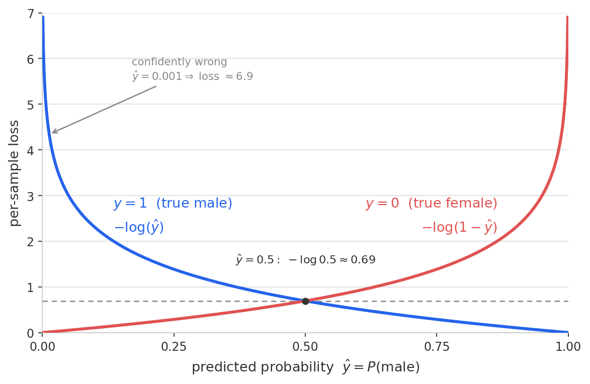
In practice, \(\hat{y}\) is clamped away from 0 and 1 by a small epsilon (here \(10^{-15}\)) to avoid \(\log(0) = -\infty\).

Where it comes from. Binary cross-entropy is not an arbitrary choice — it falls out of maximum likelihood. The model treats each label as a Bernoulli draw with probability \(\hat{y}_i\):

\[P(y_i \mid x_i) = \hat{y}_i^{\,y_i}\,(1 - \hat{y}_i)^{1 - y_i}\]

The exponents act as a switch: the expression is \(\hat{y}_i\) when \(y_i = 1\) and \(1 - \hat{y}_i\) when \(y_i = 0\). Assuming the samples are independent, the likelihood of the whole dataset is the product \(\prod_{i=1}^{m} P(y_i \mid x_i)\). Taking the log turns the product into a sum, then negating and averaging gives:

\[-\frac{1}{m} \sum_{i=1}^{m} \left[ y_i \log \hat{y}_i + (1 - y_i) \log(1 - \hat{y}_i) \right]\]

which is exactly the loss above. Minimizing it is the same as finding the weights that make the observed labels most probable — maximum likelihood estimation.

gradient descent

To minimize the loss we need its gradient with respect to the weights — the direction of steepest increase, which we step against. Starting from the chain rule:

\[\frac{\partial \mathcal{L}}{\partial \tilde{w}_j} = -\frac{1}{m} \sum_{i=1}^{m} \left[ \frac{y_i}{\hat{y}_i} - \frac{1 - y_i}{1 - \hat{y}_i} \right] \frac{\partial \hat{y}_i}{\partial \tilde{w}_j}\]

The sigmoid derivative is \(\frac{\partial \sigma}{\partial z} = \sigma(z)(1 - \sigma(z)) = \hat{y}_i(1 - \hat{y}_i)\), so:

\[\frac{\partial \hat{y}_i}{\partial \tilde{w}_j} = \hat{y}_i(1 - \hat{y}_i)\, \tilde{x}_{ij}\]

Substituting and simplifying:

\[\frac{\partial \mathcal{L}}{\partial \tilde{w}_j} = -\frac{1}{m} \sum_{i=1}^{m} \left[ y_i(1 - \hat{y}_i) - (1 - y_i)\hat{y}_i \right] \tilde{x}_{ij} = \frac{1}{m} \sum_{i=1}^{m} (\hat{y}_i - y_i)\, \tilde{x}_{ij}\]

In matrix form:

\[\nabla_{\tilde{w}} \mathcal{L} = \frac{1}{m} \tilde{X}^\top (\hat{y} - y)\]

This is identical in form to the linear regression gradient — residuals projected back through the feature matrix. The sigmoid derivative \(\hat{y}(1 - \hat{y})\) cancels exactly with the denominator from the log inthe loss. This is not a coincidence: binary cross-entropy was designed to pair with the sigmoid precisely because of this cancellation. It gives clean gradients even when the model is confidently wrong.

The update rule is the same as before:

\[\tilde{w} \leftarrow \tilde{w} - \alpha \nabla_{\tilde{w}} \mathcal{L}\]

One epoch is one full pass through the training data, computing this gradientand updating the weights. We repeat for thousands of epochs until the loss stops decreasing.

normalizing features

Same approach as in linear regression — means and standard deviations are computed from the training set only and reapplied without recomputing during predict(). Computing them from the full dataset before splitting leaks validation information into training.

metrics

Logistic regression outputs a probability, not a ring count — RMSE and R² measure distance from a continuous target and are meaningless here.

Binary cross-entropy is the training loss, covered in the loss function section above.

Accuracy is the evaluation metric — the fraction of samples classified correctly after thresholding at 0.5:

\[\text{accuracy} = \frac{1}{m} \sum_{i=1}^{m} \mathbf{1}[\text{class}(\hat{y}_i) = y_i]\]

Accuracy has a known weakness on imbalanced datasets: a model that always predicts the majority class achieves high accuracy without learning anything. The abalone sex split is 54% male / 46% female — close enough to balanced that accuracy is a fair metric here. A model stuck at 54% is not learning; it is predicting the prior.

k-fold cross-validation

Same mechanism as in linear regression, with \(k = 5\). The only change is the metric: instead of minimizing RMSE, we maximize accuracy. The cross-validation function is generic over the scoring metric via a closure — no structural change was needed to support classification.

regularization

Same L1 and L2 penalties as in linear regression, with one difference: the regularization term is scaled by \(\frac{\lambda}{m}\) rather than bare \(\lambda\):

\[\nabla_{\tilde{w}} \mathcal{L}_\text{reg} = \nabla_{\tilde{w}} \mathcal{L} + \frac{\lambda}{m} \cdot \begin{cases} w_j & \text{L2} \\ \text{sign}(w_j) & \text{L1} \end{cases}\]

The gradient already divides by \(m\), so the penalty must be on the same scale. Without this, the effective regularization strength would grow with dataset size.

grid search

Same procedure as in linear regression, searching 30 log-spaced \(\lambda\) values from \(10^{-6}\) to \(10^{1}\) via 5-fold cross-validation. The only difference: we select the \(\lambda\) with the highest average validation accuracy rather than the lowest RMSE — the optimization direction flips for classification.

a note on running time. with \(\alpha = 0.01\) and 5,000 epochs, a single training run converges in a few seconds in the browser. grid search trains 5 models per \(\lambda\) across 30 values — use the cv epochs slider (default: 5,000) to control the cost. fewer iterations are enough to rank \(\lambda\) values reliably without full convergence.

interpreting this run

Learning rate α = 0.01 · 5,000 epochs · L2 regularization · best λ = 0.356 found by grid search

Loss evolution

The loss starts at 0.693 — exactly \(\ln 2\), the binary cross-entropy of a model that assigns 0.5 to every sample regardless of its features. This is the random-guess baseline for a balanced binary problem, and it is where logistic regression begins: all weights at zero, all predictions at 0.5.

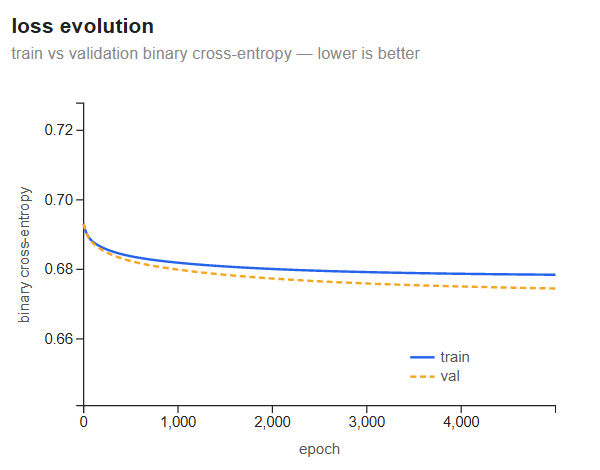
Both curves drop steeply in the first few hundred epochs, then flatten. By epoch 5,000 training loss sits around 0.680 and validation loss around 0.675 — a reduction of only ~0.013 from the baseline. The model is learning something, but not much. The validation loss ending slightly below training loss is not a sign of exceptional generalization; it reflects the 80/20 split landing slightly easier samples in the validation set.

Accuracy evolution

Accuracy starts around 53% — the majority-class prior — and climbs slowly to ~57% (train) and ~58% (val) by epoch 5,000. The curves track each other closely throughout: there is no overfitting gap. When train and val accuracy are nearly identical, it means the model has not memorized the training data — it simply has not found much signal to memorize.

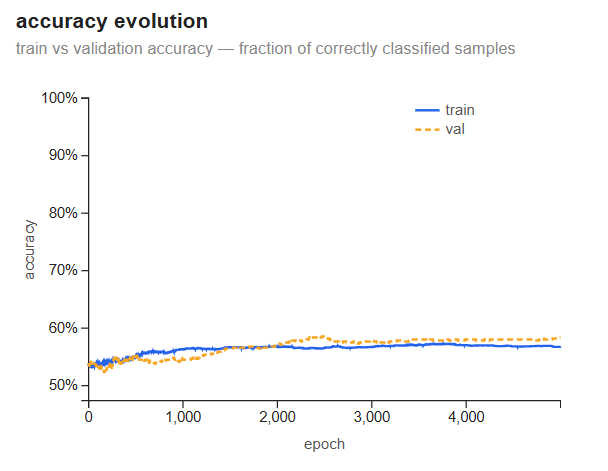
Both curves are still slowly rising at epoch 5,000, so the model has not fully converged. But the trajectory makes clear that more training would bring marginal gains — the ceiling is in the data, not the iteration count.

Predicted probabilities

Each dot is one abalone. The x-axis is P(male); the two rows separate actual males (blue, top) from actual females (red, bottom). The dashed line at 0.5 is the decision boundary.

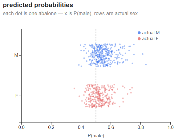
The separation is real but weak. The male distribution is centered around 0.55 and the female distribution around 0.45 — correctly shifted to opposite sides of the threshold, but with massive overlap. Most predictions fall in the 0.4–0.6 band; the model is rarely confident. This is what a ~58% accuracy ceiling looks like in probability space: not a failure to learn, but an honest reflection of how much the two classes overlap in the feature space.

Feature weights

Each bar shows the weight assigned to that feature after training. Positive weights increase P(male); negative weights decrease it.

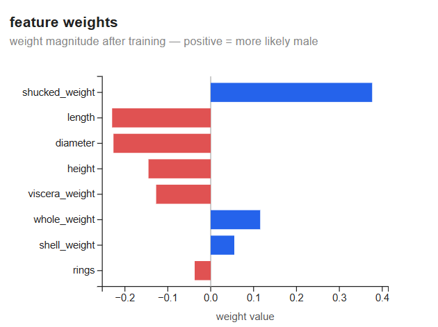
shucked_weight is the dominant positive predictor (~+0.38), with the other size and weight features carrying smaller negative weights. These signs are correlational, not causal: the physical measurements are highly collinear, so individual weights can shift or flip with small changes in the data and shouldn’t be read as biological mechanisms. The pattern is consistent with sex being weakly and diffusely encoded across overall body size — no single measurement isolates it. rings is near zero — age contributes almost nothing to sex prediction once size is accounted for.

Grid search — λ vs validation accuracy

The curve is completely flat: every λ from \(10^{-6}\) to \(10^{1}\) gives the same ~56% validation accuracy. The best λ = 0.356 is selected by the grid search but the margin over any other value is negligible.

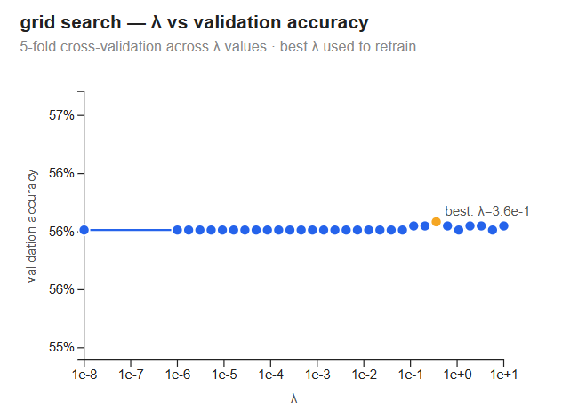
A flat grid search is an honest result: regularization only helps when the model is overfitting — fitting noise in the training data that does not generalize. Here the model is underfitting. It has not found enough signal to overfit in the first place, so there is nothing for regularization to correct. Any λ gives the same result.

Weight stability across folds

Each row shows the distribution of a feature’s weight across the 5 CV folds.

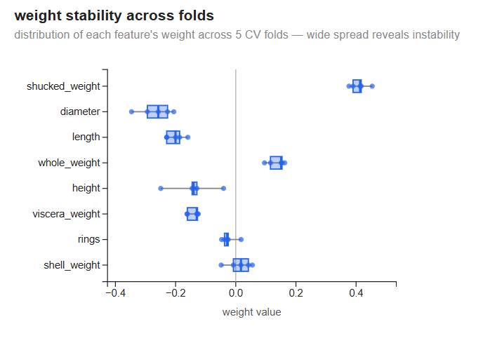
These weights come from the 5 cross-validation refits, so their magnitudes differ slightly from the single-split run above (e.g. shucked_weight ~+0.43 here vs ~+0.38 there). Most features are remarkably stable: shucked_weight clusters tightly around +0.43, diameter and length around −0.2, whole_weight around +0.13. height shows the most spread — its whiskers extend from around −0.25 to near zero, making it the least reliable signal. This is not multicollinearity in the same dramatic sense as the linear regression weights — no feature is being pushed to opposite extremes across folds. The model is consistent; it is just consistently uncertain about the target.

where logistic regression falls short

58% accuracy on a near-balanced binary problem means the model is correctly classifying only 4 out of 100 more samples than the majority-class baseline — always predicting male — would. Three factors explain this:

The boundary is linear. Logistic regression draws a single flat hyperplane through the feature space. If the true relationship between physical measurements and sex is nonlinear — and biology suggests it is — no choice of weights can capture it.

The features overlap. Males and females share nearly identical distributions across all eight measurements. shucked_weight is the strongest signal, but even it shows heavy overlap. The classes are not linearly separable, and may not be separable at all with these features.

Sex is hard to predict from morphology alone. The abalone dataset was collected for age estimation, not sex classification. The features it contains — size, weight, rings — are proxies for age, not sex. A dedicated study would collect gonad measurements, spawning observations, or genetic markers.

This is not a failure of the implementation. It is an honest result: the model correctly tells us that sex cannot be reliably inferred from these physical measurements with a linear classifier. That is useful to know.

references

James, G., Witten, D., Hastie, T., Tibshirani, R., and Taylor, J. An Introduction to Statistical Learning with Applications in Python. Springer, 2023. §4.3 (logistic regression), §6.2 and §6.4 (regularization).
Hastie, T., Tibshirani, R., and Friedman, J. The Elements of Statistical Learning, 2nd ed. Springer, 2009. §4.4 (logistic regression), §3.4 (regularization).
Géron, A. Hands-On Machine Learning with Scikit-Learn, Keras, and TensorFlow, 3rd ed. O’Reilly, 2022. Chapter 4 (training models).
Goodfellow, I., Bengio, Y., and Courville, A. Deep Learning. MIT Press, 2016. Chapter 3 (information theory and cross-entropy).
Logistic Regression — GeeksForGeeks
Binary Cross Entropy — Towards Data Science