ferrolearn #3 — k-nearest neighbors

The first two models in this series learned a set of weights: linear and logistic regression both ran gradient descent to fit parameters, then threw the training data away. K-nearest neighbors does the opposite. It learns nothing — no weights, no equation, no optimization. It keeps the training data around and classifies a new point by looking at the examples nearest to it. This makes it the simplest model in the series to state and, in some ways, the most different.

We apply it to the abalone dataset, predicting sex from physical measurements. Unlike the logistic regression post, which dropped infants to get a binary problem, here we keep all three categories — M, F, and I — because majority voting handles any number of classes without changing anything. That makes this the first genuinely multi-class problem in the series.

→ open the interactive demo

the model

The idea is simple. To classify a new abalone, we find the \(k\) training abalone most similar to it, and let them vote — the majority class among those \(k\) neighbors is the prediction.

“Most similar” means closest in feature space. We measure closeness with Euclidean distance — the straight-line distance between two points across all \(n\) features:

\[d(\mathbf{x}, \mathbf{x}_i) = \sqrt{\sum_{j=1}^{n} (x_j - x_{ij})^2}\]

where \(\mathbf{x}\) is the point we want to classify and \(\mathbf{x}_i\) is one training sample. We compute this distance to every training point, sort ascending, take the \(k\) smallest, and return the most common label among them:

\[\hat{y} = \text{mode}\{\, y_{(1)}, y_{(2)}, \ldots, y_{(k)} \,\}\]

where \(y_{(1)}, \ldots, y_{(k)}\) are the labels of the \(k\) nearest neighbors. Because it is just a count, this generalizes to three classes — or thirty — with no extra machinery, which is why we can keep infants in the problem.

No training, no parameters. This is the defining feature of KNN. There is no gradient descent, no loss function, nothing to minimize. fit() only stores the (normalized) training data; all the actual work happens at prediction time, when the distances are computed. This style is called lazy or instance-based learning: the model is the training set. It is the mirror image of the regression models, which spent all their effort in fit() and then predicted instantly.

The decision boundary is jagged. KNN never writes down a boundary, but one exists implicitly. If you colored every point in feature space by the class KNN would assign it, you would see regions — one per class — and the borders between them are not straight. They bend and wander around individual training points. At \(k=1\) the regions are the Voronoi cells around each training sample, maximally irregular; as \(k\) grows they smooth out. This is the sharp contrast with logistic regression, whose boundary is always a single flat hyperplane. KNN can carve arbitrary, curved regions — it trades the linear model’s rigidity for flexibility. As we will see, that flexibility is also its weakness.

regression, too. KNN is not only a classifier. To predict a continuous target — ring count, say — you swap the majority vote for the mean of the \(k\) neighbors’ values. Everything else stays identical. This post stays on classification, but the same code is one line away from the regression setting.

distance and normalization

Euclidean distance sums contributions from every feature, which means a feature’s scale decides how much it matters. The abalone measurements live on very different scales — weights in grams, lengths in millimetres, ring counts as integers up to 29 — so without rescaling, whichever feature has the largest numeric range would dominate the distance and effectively pick the neighbors on its own. The others would barely register.

KNN is therefore even more sensitive to feature scaling than the gradient-descent models, where scaling only affected convergence speed. Here it changes the answer. So we standardize every feature to zero mean and unit variance before computing any distance:

\[z = \frac{x - \mu}{\sigma}\]

Here \(\mu\) is the feature’s mean and \(\sigma\) its standard deviation, both measured across the training samples. Subtracting \(\mu\) recenters the feature on zero; dividing by \(\sigma\) rescales it so one unit equals one standard deviation. The transformed value \(z\) then reads as “how many standard deviations above or below average this measurement is” — a common language every feature speaks, whether it started out as grams, millimetres, or ring counts.

data leakage. as in the regression posts, \(\mu\) and \(\sigma\) are computed from the training set only and reapplied to the test data without recomputing — see linear regression. Computing them from the full dataset would leak information about the held-out points into the model.

With every feature on the same scale, a millimetre of length and a gram of shell weight contribute comparably to the distance, and the neighbors are chosen on overall similarity rather than on whichever column happened to have the biggest numbers.

choosing k

\(k\) — the number of neighbors — is the model’s only knob, and it controls the bias–variance tradeoff directly and visibly.

Small \(k\) makes the model sensitive to individual points. At \(k=1\), each prediction is simply the label of the single closest training sample; the decision regions are the jagged Voronoi cells described above. This fits the training data perfectly — including its noise — which is high variance: move one training point and the boundary shifts. On unseen data it is brittle.

Large \(k\) averages over a wide neighborhood. The boundary smooths, small local structures wash out, and in the limit \(k \to m\) every query just returns the global majority class. That is high bias: the model is too rigid to follow the real structure.

The right \(k\) sits between these extremes, and we find it by cross-validation rather than by guessing.

Ties. With two classes an odd \(k\) can never tie, but with three (M, F, I) it still can — \(k=5\) might split 2–2–1. We break such ties toward the nearest neighbor: among the classes with the top count, the one whose closest member is nearest wins. This keeps predictions deterministic and gently favors the more similar class.

k-fold cross-validation

We cannot choose \(k\) by training accuracy, and KNN makes the reason especially stark: because the model is the training set, predicting on the training data lets every point find itself as its own nearest neighbor (distance zero). At \(k=1\) that gives 100% training accuracy — a number that says nothing about how the model generalizes.

So we evaluate on held-out data. The mechanism is the same k-fold cross-validation used in the regression posts: split the data into 5 folds, and for each candidate neighbor count, train on the other 4 folds and score on the held-out one, then average the 5 scores. That average is a single held-out estimate of how well that value of \(k\) generalizes.

We compute that estimate for every candidate \(k\) and keep the one with the highest average validation accuracy — that is how \(k\) is chosen. The sweep across all candidates is exactly what the grid search (next section) plots, and the winning \(k\) is the value used for every figure that follows.

One naming collision is worth flagging: the \(k\) in “k-nearest neighbors” (the number of neighbors) is not the \(k\) in “k-fold” (the number of folds). We use 5 folds to choose the best number of neighbors.

grid search

To pick the neighbor count automatically, we sweep a range of values, score each by its average validation accuracy across the folds, and keep the best. It is the same procedure as the \(\lambda\) grid search in the earlier posts — only the hyperparameter has changed: we are searching over the number of neighbors instead of a regularization strength, and selecting the value with the highest validation accuracy.

a note on running time. KNN flips the cost structure of the series. There is no training loop — fit() just stores the data — but every prediction compares the query against all \(m\) training points, so scoring a whole set is \(O(m^2)\). That makes the grid search, which re-scores across folds and neighbor counts, the expensive part. Reduce the k max or cv folds sliders if you want faster results; raise them for a finer search.

interpreting this run

k = 39 found by grid search · 5-fold cross-validation

The chosen model gets a little over half of the held-out abalone right — about 54% overall — but that single number averages three very different outcomes, so it is worth reading class by class.

Confusion matrix

Rows are the actual class, columns the predicted class; each row sums to 100%, and a darker diagonal means better classification.

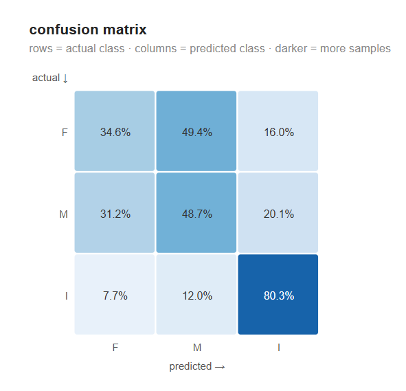
One row behaves; two do not. Infants land on the diagonal 80.3% of the time, leaking only slightly to M (12.0%) and F (7.7%). The male and female rows tell the opposite story: just 48.7% of males and 34.6% of females are labeled correctly, and the misses pile up between M and F rather than spilling into I. The most revealing cell is the top middle — actual females are called male 49.4% of the time, more often than they are called female. And the F and M rows are near-copies of each other (34.6 / 49.4 / 16.0 versus 31.2 / 48.7 / 20.1), exactly what you would expect if the two sexes sit in the same region of feature space: a point’s neighbors are a mix of both, and the vote tips toward whichever is locally denser.

Per-class accuracy

The fraction of samples correctly classified within each sex category — this is the diagonal of the confusion matrix, read one class at a time.

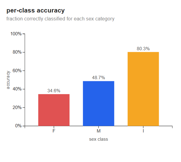
The gap is the whole result. Infants (~80%) are easy: smaller and lighter across every measurement, so their nearest neighbors are almost all other infants. Adults are not — males (~49%) and females (~35%) overlap so heavily that even 39 neighbors cannot pull them apart, and the model is barely better than a coin flip between the two. The asymmetry matters too: females do worse than males because M is the more common adult class, so wherever the neighborhood is mixed the majority vote leans male and the females pay for it.

Prediction distribution

For each actual class, where the model’s predictions land — the off-diagonal dots are where confusion happens.

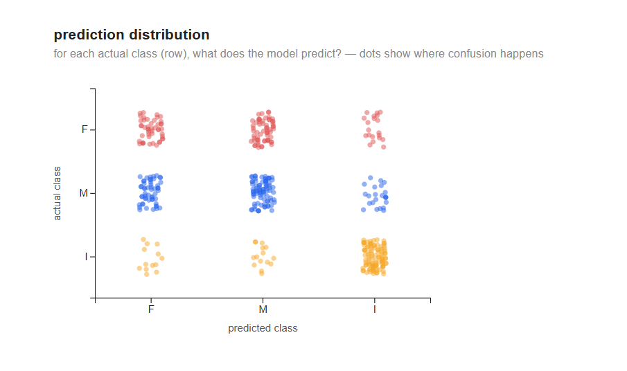
The same story, as dots instead of percentages. The bottom row — actual infants — collects into the I column with only a thin scatter elsewhere. The top two rows spread almost evenly across the F and M columns, with just a light tail into I. There is no tight diagonal for the adults; the off-diagonal cells are nearly as full as the on-diagonal ones. That is the signature of an honest failure, not a buggy one: the model makes the same structured mistake everywhere — confusing the two adult sexes — because the measurements genuinely do not separate them.

Grid search — k vs validation accuracy

Cross-validation accuracy across the candidate neighbor counts, with the best \(k\) highlighted.

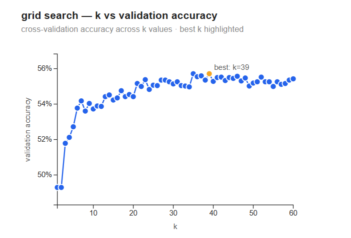
This is the bias–variance tradeoff in a single curve. At \(k=1\) accuracy sits around 49% — each prediction just copies its single nearest neighbor, noise included. (Note it is ~49%, not the 100% you would get by scoring on the training data; the held-out split keeps it honest.) Accuracy rises steeply as \(k\) grows and the vote begins averaging out that noise, then flattens into a broad plateau from about \(k=20\) on, peaking at \(k=39\) near 55.7%. The plateau is nearly flat — \(k=39\) is barely ahead of \(k=25\) or \(k=55\) — so the exact winner is not meaningful; what matters is that the model needs a large neighborhood to do its best. That is itself a finding: local structure is too noisy to trust, so the model does better polling dozens of neighbors than a few. Push \(k\) higher still and the curve drifts back down, as the neighborhood grows wide enough to wash out real structure — the underfitting end of the tradeoff.

where KNN struggles

Every feature counts equally. Distance treats all features the same, so an irrelevant or noisy feature adds noise to every comparison. A linear model can drive a useless coefficient to zero; KNN has no such mechanism — it cannot down-weight a feature, only be dragged around by it. Careful feature selection and scaling matter more here than in any model so far.

No model, no explanation. KNN returns predictions but learns no structure. There are no weights to interpret, no equation, nothing to tell you why two sexes are hard to separate — only that the neighbors disagreed. The regression posts at least handed us coefficients to argue over; KNN hands us nothing but the data itself.

The cost lives at prediction time. Lazy learning has a price: there is no compact model to ship, and every prediction scans the whole training set. Cost grows with the data, exactly where the regression models stayed constant.

None of this makes KNN a bad choice — on the right problem, with few, well-scaled, relevant features, a model that simply asks “what do the nearest examples look like?” is hard to beat. It just asks more of the data, and of us, than a model that compresses everything into a handful of weights.

references

Russell, S. and Norvig, P. Artificial Intelligence: A Modern Approach, 4th ed. Pearson, 2021. §12.6 (nearest-neighbor models), §19.7.1 (nonparametric classification).
James, G., Witten, D., Hastie, T., Tibshirani, R., and Taylor, J. An Introduction to Statistical Learning with Applications in Python. Springer, 2023. §3.5 (KNN regression), §4.4.4 (KNN classification).
K-Nearest Neighbor (KNN) Algorithm — GeeksForGeeks
The Bias-Variance Tradeoff — Towards Data Science