ferrolearn #1 — linear regression
Linear regression is where every ML course starts, and for good reason — it is the simplest model that is still useful. But simple does not mean trivial. Implementing it from scratch forces you to confront questions that libraries hide: how do you normalize without leaking information? why does the gradient look the way it does? when does regularization actually help?
This post covers the implementation I wrote in Rust (compiled to WASM) for the ferrolearn series, applied to the abalone dataset — predicting the number of rings (a proxy for age) from physical measurements.
the model
Linear regression assumes the target is a linear combination of the input features plus a bias term:
\[\hat{y} = \beta_0 + \beta_1 x_1 + \beta_2 x_2 + \cdots + \beta_p x_p\]To keep the math clean, we absorb the bias into the weight vector by prepending a column of ones to the feature matrix — a technique called bias augmentation. Without it, we have two separate objects to optimize: a weight matrix \(W \in \mathbb{R}^{m \times n}\) and a bias vector \(b \in \mathbb{R}^m\). With it, we stack them into one:
\[\tilde{X} = \begin{bmatrix} 1 & x_{11} & \cdots & x_{1n} \\ 1 & x_{21} & \cdots & x_{2n} \\ \vdots & \vdots & \ddots & \vdots \\ 1 & x_{m1} & \cdots & x_{mn} \end{bmatrix} \in \mathbb{R}^{m \times (n+1)}, \qquad \tilde{w} = \begin{bmatrix} w_0 \\ w_1 \\ \vdots \\ w_n \end{bmatrix} \in \mathbb{R}^{n+1}\]\(\tilde{X}\) is a matrix with \(m\) rows (one per sample) and \(n+1\) columns (one per feature, plus the leading ones column). \(\tilde{w}\) is a vector of \(n+1\) weights, where \(w_0\) is the bias and \(w_1, \ldots, w_n\) are the feature weights. The prediction for all samples at once is then the matrix-vector product \(\hat{y} = \tilde{X}\tilde{w} \in \mathbb{R}^m\) — one number per sample. This gives us the augmented form:
\[\hat{y} = \tilde{X}\tilde{w}\]where \(\tilde{X} \in \mathbb{R}^{m \times (n+1)}\) has a leading ones column and \(\tilde{w} \in \mathbb{R}^{n+1}\) holds the bias as its first element. There is now only one vector to optimize — no separate bias term to track.
We measure fit with the mean squared error, carrying a factor of ½ that cancels the 2 from differentiating the square and keeps the gradient clean:
\[\mathcal{L} = \frac{1}{2m} \sum_{i=1}^{m} (\hat{y}_i - y_i)^2 = \frac{1}{2m}\|\tilde{X}\tilde{w} - y\|^2\]A geometric view. Minimizing squared error has a clean geometric meaning. Picture the target vector \(y\) and every prediction the model could make — all of \(\tilde{X}\tilde{w}\) as \(\tilde{w}\) ranges over weight space. Those reachable predictions form a flat subspace: the column space of \(\tilde{X}\). Least squares finds the point in that subspace closest to \(y\) — the orthogonal projection of \(y\) onto it. The residual \(y - \hat{y}\) is what’s left over, sticking out perpendicular to the subspace: it is everything about \(y\) that no linear combination of the features can reach. Gradient descent walks toward that projection one step at a time; the normal equation jumps straight to it.
gradient descent
To minimize \(\mathcal{L}\) we need to know which direction to move the weights to make the error smaller. The gradient tells us exactly that — it is a vector that points in the direction of steepest increase of the loss, so we step in the opposite direction. Concretely, for each weight \(\tilde{w}_j\), the gradient tells us: “if you increase this weight slightly, does the error go up or down, and by how much?”
The gradient of the loss with respect to the weights is:
\[\nabla_{\tilde{w}} \mathcal{L} = \frac{1}{m} \tilde{X}^\top (\tilde{X}\tilde{w} - y)\]We divide by \(m\) (the number of samples) so the gradient magnitude does not grow with dataset size — without this, a dataset twice as large would produce steps twice as large, requiring a different learning rate for every dataset.
The update rule is applied once per epoch — one full pass through the training data:
\[\tilde{w} \leftarrow \tilde{w} - \alpha \nabla_{\tilde{w}} \mathcal{L}\]An epoch is one complete cycle where every training sample has contributed to a gradient update. We repeat this process for hundreds or thousands of epochs, nudging the weights a little each time until the loss stops improving.
\(\alpha\) is the learning rate — a small positive number (typically between 0.0001 and 0.1) that controls how large each step is. Too large and the weights overshoot the minimum, causing the loss to oscillate or diverge. Too small and convergence is needlessly slow. It is a hyperparameter: we set it before training, not learned from data.
Why this works at all. Mean squared error is a convex function of the weights — its loss surface is a single smooth bowl with one lowest point and no others. That is what makes gradient descent safe here: wherever the weights start, following the slope downhill leads to the same global minimum, with no local minima to get trapped in and no dependence on initialization. It is why we can set every weight to zero at the start and still converge. Many models later in this series — neural networks especially — give this up: their loss surfaces are riddled with local minima, and where you start genuinely matters.
Note that we never compute \((\tilde{X}^\top \tilde{X})^{-1} \tilde{X}^\top y\) — the closed-form normal equation. It gives the exact optimum in one step but requires inverting an \((n+1) \times (n+1)\) matrix, which is \(O(n^3)\) and numerically unstable for correlated features. Gradient descent scales to large \(n\) and adapts naturally to regularization.
Two features are correlated when they carry redundant information — knowing one tells you a lot about the other. In the abalone dataset, length, diameter, and height are all measurements of physical size and move together: a longer shell is almost always also wider and taller. Similarly, whole_weight, shucked_weight, viscera_weight, and shell_weight are all mass measurements of the same animal split different ways — they are nearly interchangeable.
When features are correlated, the normal equation \((\tilde{X}^\top \tilde{X})^{-1} \tilde{X}^\top y\) becomes unreliable because \(\tilde{X}^\top \tilde{X}\) is nearly singular — it has no unique inverse. Intuitively: if two columns of \(\tilde{X}\) are nearly identical, the matrix cannot tell them apart, and there are infinitely many weight combinations that produce the same predictions. The inversion amplifies tiny numerical errors into wildly different weight values. Gradient descent sidesteps this entirely — it never inverts anything, it just follows the slope.
normalizing features
Raw features in the abalone dataset span very different scales: lengths are in millimetres (0–1), weights are in grams (0–3), rings are integers (1–29). Without normalization, gradient descent would take enormous steps along the weight dimension and tiny steps along the length dimension — convergence would be slow or divergent.
We standardize each feature to zero mean and unit variance:
\[z = \frac{x - \mu}{\sigma}\]But there is a subtle trap here.
data leakage. \(\mu\) and \(\sigma\) must be computed from the training set only. If you compute them from the full dataset before splitting, information from the validation set bleeds into the training process — the model appears to generalize better than it does. In the Rust implementation,
column_meansandcolumn_stdsare called insidefit()on the training data only, stored on the model struct, and reapplied (without recomputing) duringpredict().
encoding sex
The abalone dataset includes a categorical feature: sex (M, F, I for infant). Linear models require numerical input, so we need to encode it.
A naive approach assigns integers — M=0, F=1, I=2 — but this implies a false ordering: the model would treat “infant” as twice “female”, which is meaningless for a nominal category.
Instead we use one-hot encoding with female as the reference (dropped) category:
| sex | sex_M | sex_I |
|---|---|---|
| M | 1 | 0 |
| F | 0 | 0 |
| I | 0 | 1 |
This gives each category an independent weight. Female is the reference — its effect is captured by the intercept. Dropping one column avoids the dummy variable trap: if we kept all three, they would sum to 1 for every row, creating perfect multicollinearity with the bias column and making the system underdetermined.
metrics: R² and RMSE
The sum of squared residuals is the loss we optimize, but it is hard to interpret — SSR of 22800 in what units? Rings squared? We use two additional metrics for reporting:
Root mean squared error (RMSE) brings the error back to the original unit:
\[\text{RMSE} = \sqrt{\frac{1}{m} \sum_{i=1}^{m} (\hat{y}_i - y_i)^2}\]An RMSE of 2.3 rings means the model is off by about 2.3 rings on average — much easier to reason about.
R² (coefficient of determination) measures the fraction of variance in the target that the model explains:
\[R^2 = 1 - \frac{\sum(\hat{y}_i - y_i)^2}{\sum(y_i - \bar{y})^2} = 1 - \frac{\text{SS}_\text{res}}{\text{SS}_\text{tot}}\]\(R^2 = 1\) means perfect prediction. \(R^2 = 0\) means the model does no better than predicting the mean. Negative values mean it is actively worse than the mean — this happens in early training when weights are all zero.
k-fold cross-validation
A single train/test split can be lucky or unlucky depending on which samples end up where. K-fold cross-validation gives a more robust estimate:
- Divide the data into \(k\) equal parts (folds)
- For each fold: train on the remaining \(k-1\) folds, evaluate on the held-out fold
- Average the \(k\) validation scores
We use \(k=5\), which is the standard choice — it balances variance (more folds = more stable estimate) against computational cost (\(k\) times more training runs). With 4177 samples each fold holds ~835 validation samples, which is large enough to be representative.
In the Rust implementation, cross-validation is generic over any SupervisedModel via a factory closure — the same function is to be reused across several models: linear regression, logistic regression, and future models without modification.
regularization
When features are correlated or the model has many parameters relative to samples, the weights can grow large to fit noise. Regularization adds a penalty to the loss that discourages this:
\(\lambda \geq 0\) is the regularization strength — a hyperparameter that controls how much the penalty influences the weights. \(\lambda = 0\) means no regularization; larger values impose a stronger penalty.
L2 (Ridge) penalizes the sum of squared weights:
\[\mathcal{L}_\text{ridge} = \mathcal{L} + \lambda \sum_{j=1}^{n} w_j^2 \qquad \text{gradient term: } 2\lambda w_j\]L2 shrinks all weights towards zero smoothly. It handles correlated features by distributing weight among them rather than arbitrarily choosing one.
L1 (Lasso) penalizes the sum of absolute weights:
\[\mathcal{L}_\text{lasso} = \mathcal{L} + \lambda \sum_{j=1}^{n} |w_j| \qquad \text{gradient term: } \lambda \cdot \text{sign}(w_j)\]L1 produces sparse solutions — it drives irrelevant weights exactly to zero, effectively performing feature selection. The non-smooth absolute value means the gradient is constant regardless of weight magnitude, so small weights get pushed to zero rather than just shrunk.
Both regularizers skip the bias term (\(j=0\)) — regularizing the intercept would shift predictions towards zero, which is not what we want.
The tradeoff is the bias-variance tradeoff: increasing \(\lambda\) introduces bias (the model can no longer fit the data as closely) but reduces variance (the model is less sensitive to noise in the training set). The right \(\lambda\) is the one that minimizes validation error, found via grid search.
grid search
\(\lambda\) controls how strongly regularization penalizes large weights — but the right value depends on the data. Too small and it has no effect; too large and it shrinks all weights towards zero regardless of their predictive value. Grid search finds the best \(\lambda\) automatically: we evaluate a range of values using 5-fold cross-validation and pick the one with the lowest average validation RMSE. The search space spans from \(10^{-6}\) to \(10^{1}\) in 30 log-spaced steps — logarithmic because the effect of regularization scales multiplicatively, not additively — plus \(\lambda = 0\) prepended as a no-regularization baseline, for 31 candidates in total.
a note on running time. with α = 0.0005 and 25,000 iterations, the final training run takes around 10–20 seconds in the browser. grid search is more expensive — it trains 5 models per λ value across 31 values, which would take several minutes at 25,000 iterations each. to keep it interactive, the demo uses a separate cv epochs slider (default: 5,000) for the cross-validation runs: fewer iterations are enough to compare λ values reliably, since CV only needs to rank them, not fully converge. if you want faster results, reduce cv epochs or the number of grid steps; if you want a more thorough search, increase them.
interpreting this run
Learning rate α = 0.0005 · 25,000 iterations · L2 regularization · best λ found by grid search
α = 0.0005 is deliberately small so gradient steps are cautious and stable; 25,000 iterations gives the model enough passes through the data to fully converge even at that slow pace.
R² evolution
This chart shows how well the model fits the data as training progresses — one point per epoch for both the training set (solid blue) and the validation set (dashed orange).
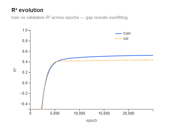
Both lines start pinned at the bottom of the chart, around −0.5 — but that is a display floor, not the real value. The y-axis is clamped at −0.5, because the first epochs sit so far below the rest of the curve that showing them would flatten everything informative. With all weights at zero, every prediction is zero, so the true starting R² is much lower — roughly −9. A negative R² means the model is worse than simply predicting the average, which makes sense at epoch 0: predicting zero for a target that averages ~10 rings is far worse than predicting the mean. A negative R² means the model is actively worse than just predicting the average, which makes sense at epoch 0: all weights are zero, so every prediction is zero — far below the ~10-ring average. As gradient descent adjusts the weights, R² climbs rapidly in the first ~3,000–5,000 iterations, then flattens. By 25,000 iterations the curves are completely flat — the model has converged and more iterations would change nothing.
The final values: training R² ≈ 0.55, validation R² ≈ 0.43. The gap between them (~0.12) is mild but real — the the model fits the training data slightly better than it fits data it has never seen — this is expected, since the model was optimized on the training set and had no information about the validation set during training. With only 9 features and 4,177 samples this is not severe overfitting; it reflects the inherent noise in ring counting more than model complexity.
RMSE evolution
RMSE measures the average prediction error in the same unit as the target — rings. It starts around 11 rings at epoch 0: with all weights at zero, every prediction is zero, so each one misses by roughly a full target value — the error is enormous. (If the model instead predicted the mean, RMSE would be the ring standard deviation, about 3.3.). It drops steeply in the first 5,000 iterations as gradient descent finds the main signal in the data, then flattens. By 25,000 iterations both curves are flat — the model has converged.
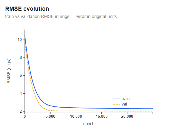
Final values: train RMSE ≈ 2.2 rings, val RMSE ≈ 2.1 rings. Notably, validation RMSE ends up slightly below training RMSE — the opposite of what you might expect. The cause is the split: it is taken contiguously (first 80% / last 20%, no shuffle), and the last fifth of the file happens to have a narrower spread of ring counts — standard deviation ≈ 2.7 versus ≈ 3.3 for the training portion. A lower-variance target is easier to predict in absolute terms, so RMSE comes out lower even though validation R² is worse (0.43 vs 0.55). It is not a sign the model generalises perfectly — shuffling before splitting would make the two sets match.
Grid search — λ vs validation RMSE
Before the final model was trained, we searched for the best regularization strength λ using 5-fold cross-validation. For each candidate λ, five models were trained on different subsets of the data and evaluated on the held-out fold. The chart shows the average validation RMSE (error in rings) across the five folds for each λ.
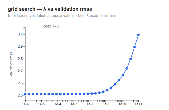
The curve is flat from λ = 10⁻⁶ to λ ≈ 10⁻², with RMSE staying around 2.50 rings. Above 10⁻², RMSE rises steeply — at λ = 10¹ it reaches ~3.0 rings. The best λ is 0 (no regularization). This is an honest result: with 9 features and ~4,000 samples the model has far more data than parameters and is not overfit, so there is nothing for regularization to fix. At high λ the penalty dominates and drives all weights towards zero regardless of their predictive value — predictions collapse towards the mean, RMSE rises.
Note that grid search used 5,000 iterations per fold rather than 25,000 — enough for the models to separate meaningfully across λ values, which is all CV needs to do.
Predicted vs actual
Each dot is one abalone. A perfect model would place every dot exactly on the diagonal dashed line.
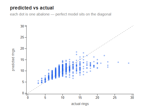
The model does well in the 5–15 ring range, where most of the dataset lives — dots cluster tightly around the diagonal. Above 15 rings the model systematically underpredicts: the diagonal keeps rising but predictions plateau around 13–15. This is not a bug; it is a fundamental limitation of linear models. Ring count grows nonlinearly with age and physical size — older abalones add rings at a slower rate relative to their size — and no linear combination of the features can capture that curve.
The vertical striping is also characteristic: ring counts are integers (3, 4, 5, …) but the model outputs continuous predictions, which cluster around the most common values in the training set.
Feature weights
Each bar shows how much a one-unit increase in that feature (after standardization) changes the predicted ring count, holding all other features constant.
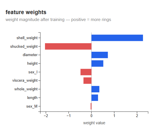
The most striking result: shell_weight has a large positive weight (~+2.3) and shucked_weight has a large negative weight (~−2.2). Both measure mass — shell_weight is the dried shell, shucked_weight is the meat. They are highly correlated with each other and with ring count. When two features carry nearly the same information, the model cannot distinguish their individual contributions — it compensates by assigning them large weights of opposite sign that partially cancel. This is called multicollinearity: the individual weights are not interpretable in isolation, but their combined effect is stable. L2 regularization would shrink both towards zero and spread the weight more evenly — but as the grid search shows, it does not improve generalization on this dataset.
sex_M is near zero — being male versus female has almost no predictive power for ring count once physical measurements are included. sex_I (infant) is negative — infants have fewer rings, as expected, since ring count is a proxy for age.
Weight stability across folds
Each row shows how much a feature’s weight varies across the 5 CV folds. A tight cluster means the model assigns that feature a consistent weight regardless of which samples it trained on — a reliable signal. A wide spread means the weight is sensitive to the specific training data — a sign of instability, often caused by multicollinearity.
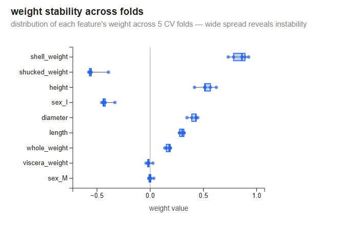
Most features are stable: shell_weight sits around +0.85, height around +0.5, diameter around +0.4, sex_I around −0.4, and shucked_weight around −0.5; the rest hug zero. The widest spreads belong to height, shell_weight, and shucked_weight — each varying by about ±0.1 across folds (shucked_weight, for instance, ranges from roughly −0.4 to −0.6, never near zero). That shell_weight and shucked_weight — the two opposite-sign mass measurements — are among the least stable is the multicollinearity effect in action: they carry overlapping information, so different training splits divide the credit between them differently.
Note that these weights come from models trained for 5,000 iterations (the CV epochs setting), not 25,000 — they are partially converged. The multicollinearity signature is already visible but less extreme than in the fully trained model above.
where linear regression breaks
Validation R² ≈ 0.43 means the model explains about 43% of the variance in ring count. The remaining 57% comes from three sources:
Nonlinearity. Physical measurements scale nonlinearly with age. A linear model draws a flat hyperplane through the data — it cannot bend to follow a curve.
Multicollinearity. The four weight measurements (whole, shucked, viscera, shell) carry heavily overlapping information. The model artificially splits them into positive and negative contributions rather than extracting a clean signal.
Biological noise. Ring counting is done by hand under a microscope and has known inter-rater variability. Some of the variance in the target is irreducible — no model can predict it because it is measurement error, not signal.
This is exactly the motivation for the next models in the series. Tree-based methods can capture nonlinearity without any manual feature engineering. Ensemble methods reduce variance by combining many models. But before going there, it is worth sitting with this result — a simple model honestly evaluated tells you more about your data than a complex model you do not understand.
references
-
James, G., Witten, D., Hastie, T., Tibshirani, R., and Taylor, J. An Introduction to Statistical Learning with Applications in Python. Springer, 2023. §3.1 (linear regression), §6.2 and §6.4 (regularization).
-
Hastie, T., Tibshirani, R., and Friedman, J. The Elements of Statistical Learning, 2nd ed. Springer, 2009. §3.1 and §3.2 (linear regression and least squares), §3.4 (regularization).
-
Géron, A. Hands-On Machine Learning with Scikit-Learn, Keras, and TensorFlow, 3rd ed. O’Reilly, 2022. Chapter 4 (training models).
source code: github.com/jjginga/ferrolearn
Enjoy Reading This Article?
Here are some more articles you might like to read next: