ferrolearn #0 — exploratory data analysis with rust + wasm
this post is part of the ferrolearn series, where i reimplement ml algorithms from my master’s course in rust + wasm.
before training a single model, you have to look at the data. not glance at it — actually look. every assumption you make about what algorithm to use, what features matter, what preprocessing is needed, lives or dies on what the data actually looks like. this first post is about that: exploratory data analysis on the abalone dataset, with all the computation running in rust compiled to webassembly.
the dataset
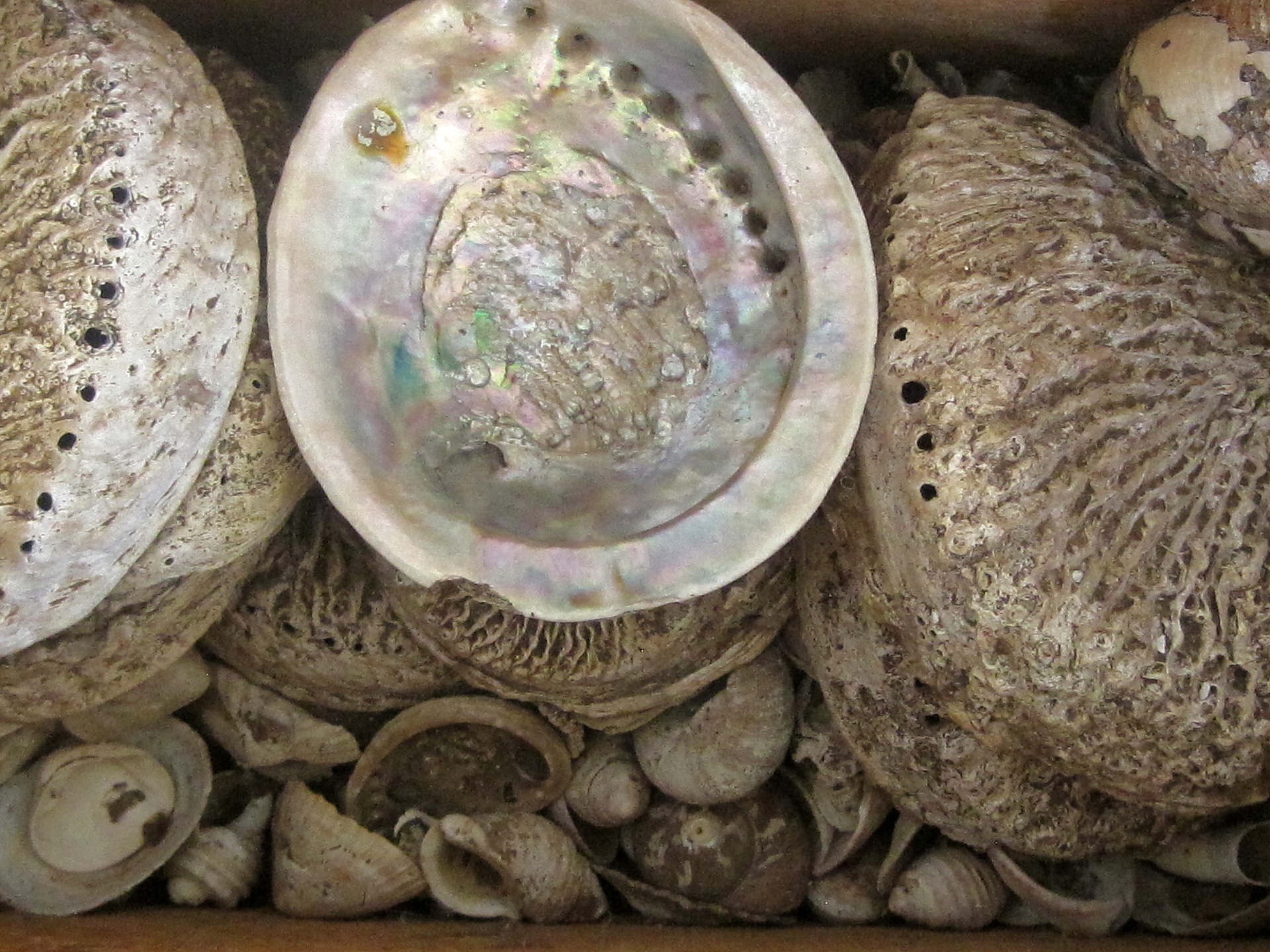
abalone are marine molluscs. they live on rocky coasts, graze on algae, and happen to have been the subject of a 1994 population biology study out of tasmania by nash, sellers, talbot, cawthorn and ford. their data has since become one of the classic regression benchmarks on the uci machine learning repository.
the problem is this: how old is an abalone? you can find out exactly by cutting the shell through the cone, staining a cross-section, and counting the growth rings under a microscope — the same way you’d age a tree. rings + 1.5 gives the age in years. but that process is slow, destructive, and requires lab equipment. the question is whether you can get a good estimate just from physical measurements taken in the field.
the dataset has 4177 samples and 8 features: sex (male, female, or infant), longest shell length, diameter perpendicular to length, height with meat in shell, whole weight, shucked weight (meat only), viscera weight (gut after bleeding), and shell weight after drying. the target is the ring count.
why eda first
a few things you can only learn by looking. is the target normally distributed or heavily skewed? are there outliers that will distort training? do features have enough variance to carry signal, or are some nearly constant? are any features so correlated that they’ll cause problems for certain models?
these aren’t rhetorical questions. the answers change what you build.
interactive demo
the eda runs entirely in rust compiled to wasm — the rust code parses the csv, computes summary statistics, and calculates the correlation matrix client-side. d3 handles the visualisation.
what the data is telling us
the target is well-behaved.
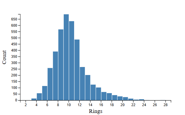
the rings histogram is roughly bell-shaped, centred around 9–10 rings (10.5–11.5 years), with a modest right tail out to 29. this is good news for linear regression — we’re not fighting a heavily skewed or bimodal target. it won’t be trivial either: there’s genuine spread, and the upper tail thins out fast, which means the model will see very few examples of old abalone.
the physical measurements are spread but not exotic.
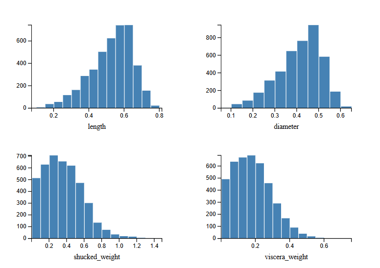
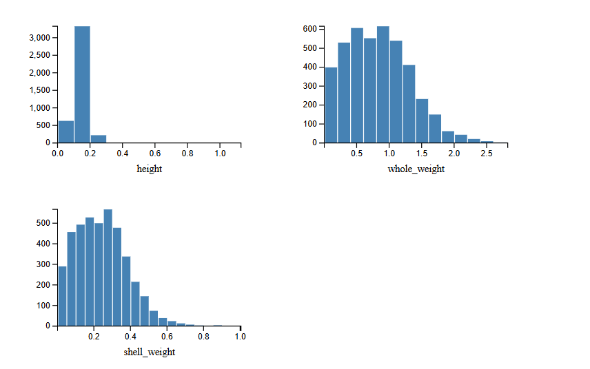
most features follow a roughly bell-shaped distribution centred on mid-range values. height stands out: there are a handful of samples with values near zero or suspiciously large. the uci page notes that missing-value examples were removed, but doesn’t mention measurement errors in height specifically. for now i’ve kept them — the rust parser validates field count and type but doesn’t filter by range — but it’s worth knowing they’re there.
the physical measurements are highly collinear.
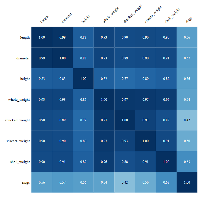
length, diameter, whole weight, shucked weight, viscera weight, and shell weight are all correlated with each other at 0.9 or higher. this is expected — bigger shells are heavier in every dimension. but it has a direct consequence for linear regression: when predictors move together this tightly, coefficient estimates become unstable. a small change in the data can produce wildly different weights. this is exactly the problem regularisation (l1 and l2) exists to solve, and it’s why we’ll spend time on it in the next post before fitting anything. shell weight ends up being the strongest individual predictor of rings — biologically sensible, since shell mass accumulates continuously over an abalone’s life.
the infant category is an age effect, not a sex effect.
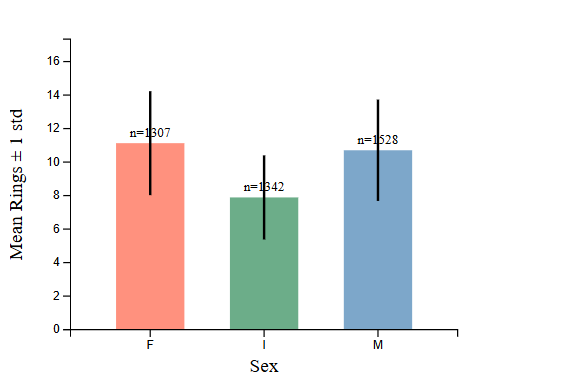
infants have systematically fewer rings than males and females. this makes biological sense — they haven’t grown as long. but it matters for modelling: sex isn’t a clean categorical feature on equal footing with the others. “I” encodes age information directly. if you one-hot encode sex naively and throw it into a regression alongside the physical measurements, you’re doubling up on age signal in a way that’s hard to reason about.
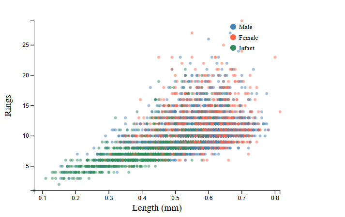
the scatter coloured by sex makes this concrete — infants cluster at the lower end of both size and ring count, while males and females overlap considerably across the full range.
what this sets up
the collinearity issue is the key takeaway going into linear regression. when predictors move together, the model can’t isolate the contribution of each one — there are infinitely many weight combinations that produce the same predictions on the training set, and tiny perturbations send the weights in different directions. l2 regularisation (ridge) addresses this by penalising large weights, shrinking correlated coefficients toward each other rather than letting them cancel out. we’ll implement gradient descent with both l1 and l2 penalties, and use cross-validation to pick the regularisation strength.
next post: linear regression, from scratch, with a gradient descent animation.
source code: github.com/jjginga/ferrolearn
Enjoy Reading This Article?
Here are some more articles you might like to read next: